GaTech - Soft Condensed Matter Lab

Home

Simulating Nematic Liquid Crystal Textures

Perry Ellis and Alberto Fernandez-Nieves

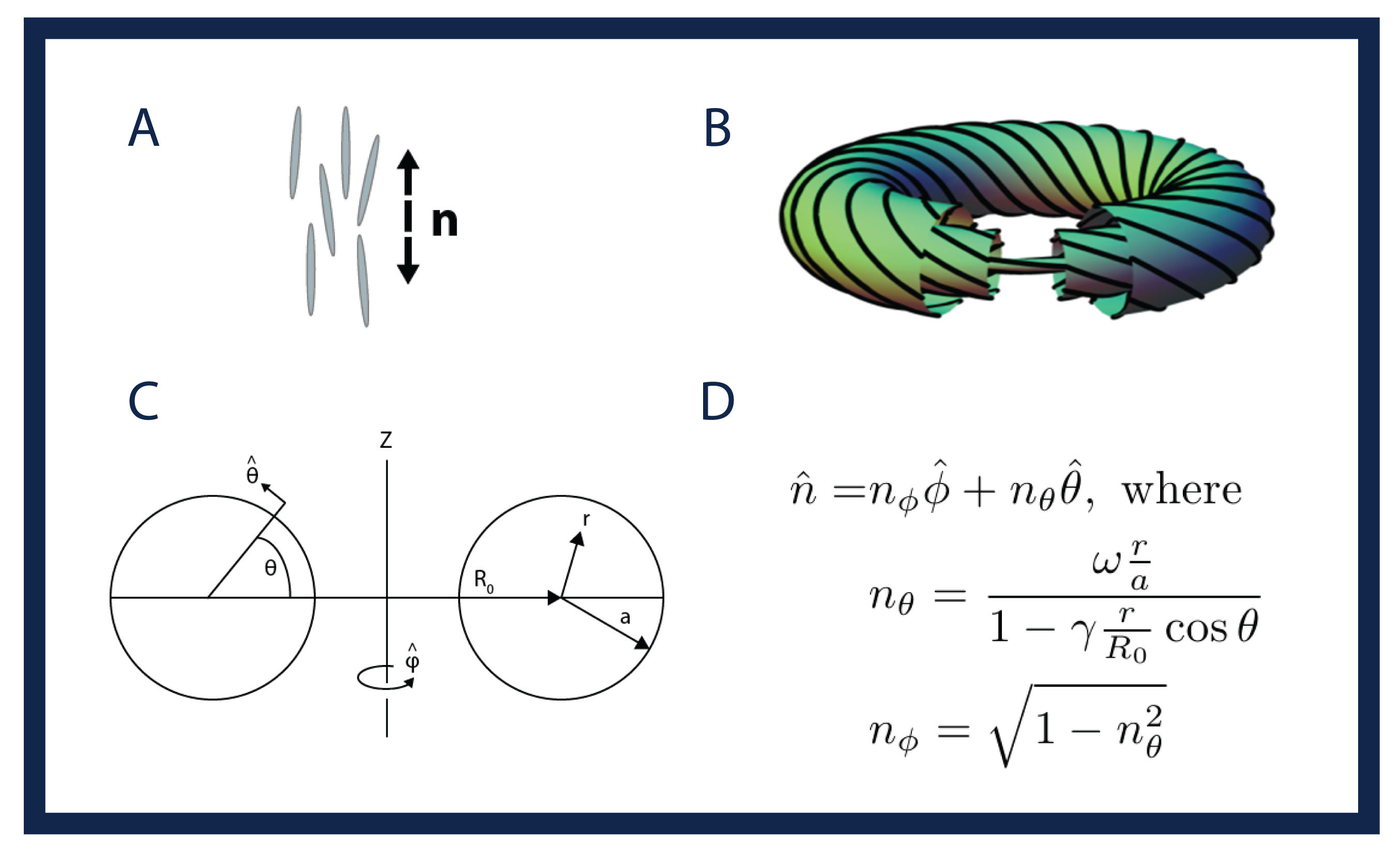
Introduction

Nematic liquid crystals are birefringent rod-like molecules that prefer to align with their long axis roughly parallel. We use the director n , an average of the orientation, to describe a nematic configuration. Under confinement in a toroidal geometry, we find that the director field exhibits a doubly-twisted structure.

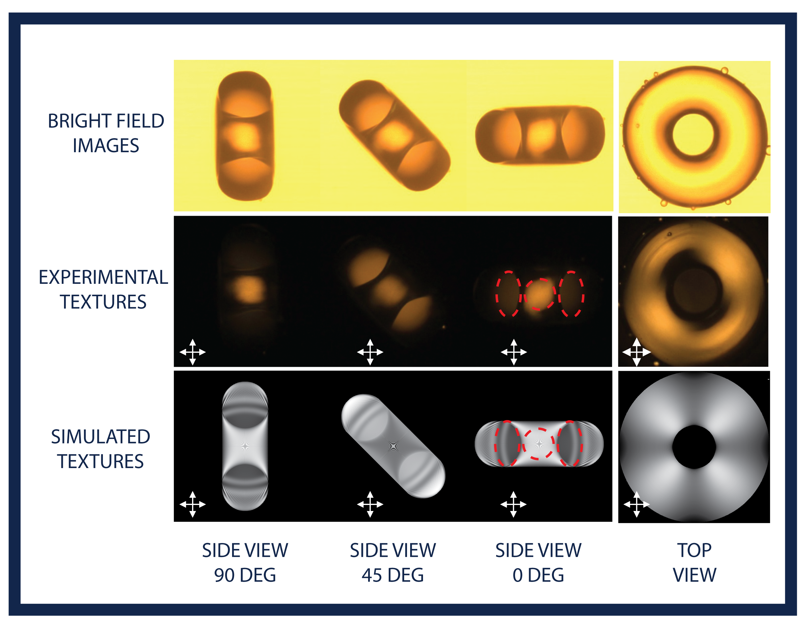
Fig. 1: (A) Schematic of nematic liquid crystal molecules aligned along the director, (B) a schematic of a toroidal drop exhibiting a double-twist strucure in the director field, (C) cross-section of a torus detailing the coordiate system used in the proposed director ansatz (D). Note that we characterize a torus by its aspect ratio, ξ = R₀/a
.

Our director ansatz incorporates this double-twist via the parameters ω and γ, which correspond to letting the director splay and twist, repsectively. We find these parameters by minimizing the Frank Free Energy including contributions from saddle-splay distortions while leaving ω and γ as free parameters. Once ω and γ are determined, we simulate crossed-polarized textures from our director ansatz and compare the simulated textures agaiunst our experimental textures. This gives us the ability to evaluate our director ansatz against our experminetal results.

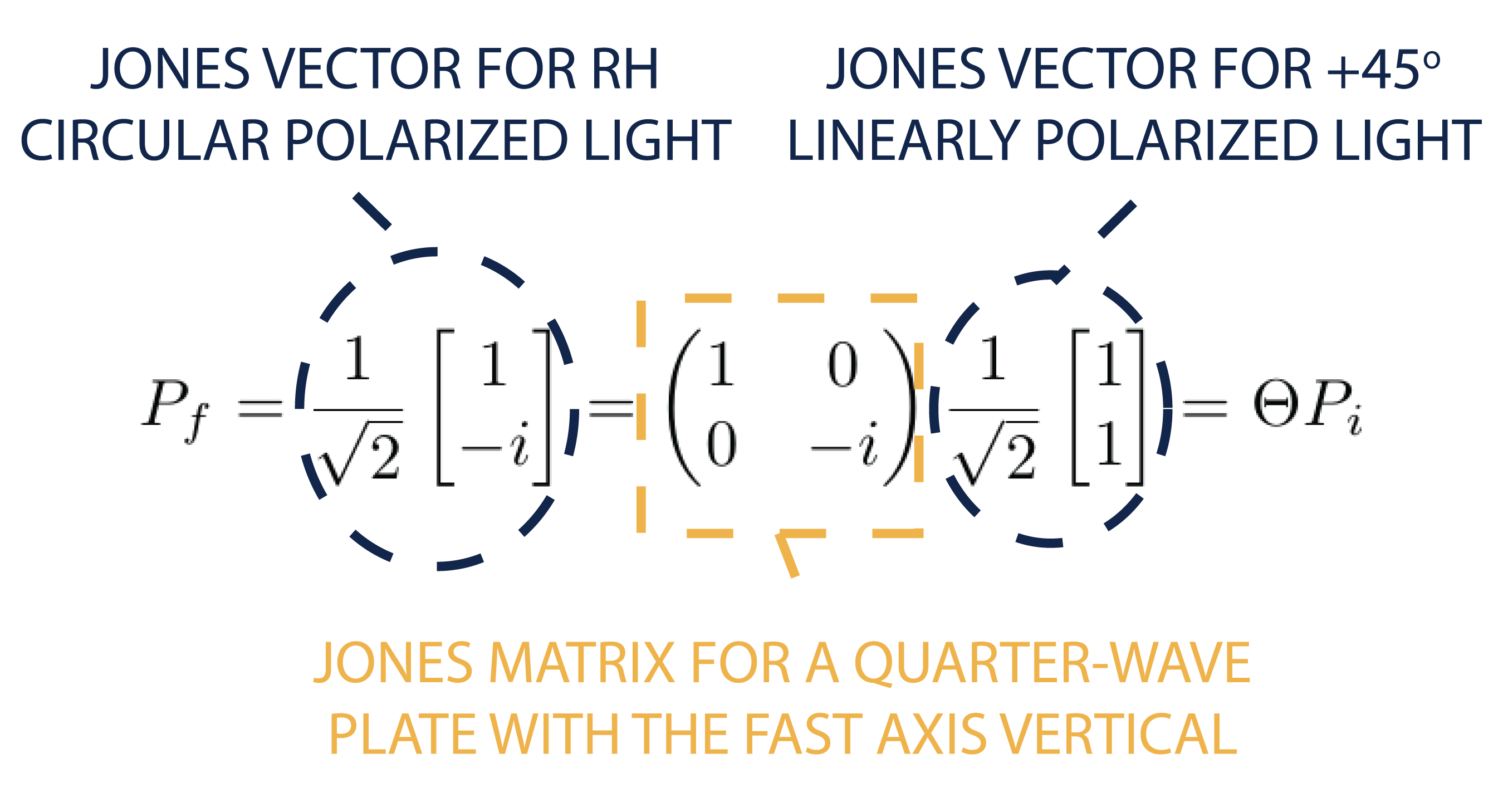
Fig. 2: Image comparison between our experimental and simulated textures for ξ = 1.8. The bright-field experimental images are included for perspective. Note how the central spot in the side-view textures is brighter than the tube when the torus is aligned at 0 degrees and how this is reversed when the torus is aligned at 45 degrees. In addition, the central spot is brigher in the textures aligned at 0 degrees than the textures aligned at 45 degrees. This qualitative behavior is seen in both the experimental and simulated textures.

Simulation Details

We simulate the crossed-polarized textures using Jones Calculus, a method of evolving and propagating polarized states through a birefringent material. Jones Calculus neglects refraction and reection, instead just treating light as a bundle of parallel rays. A polarization state is represented by a 2 x 1 Jones Vector and a birefringent element is represented by a 2 x 2 Jones Matrix. As an example, Figure 3 shows how the Jones Vector for +45 degree linearly polarized light interacts with the Jones Matrix for a quarter-wave plate with the fast axis at 0 degrees to produce an output Jones Vector of right-hand circularly polarized light.

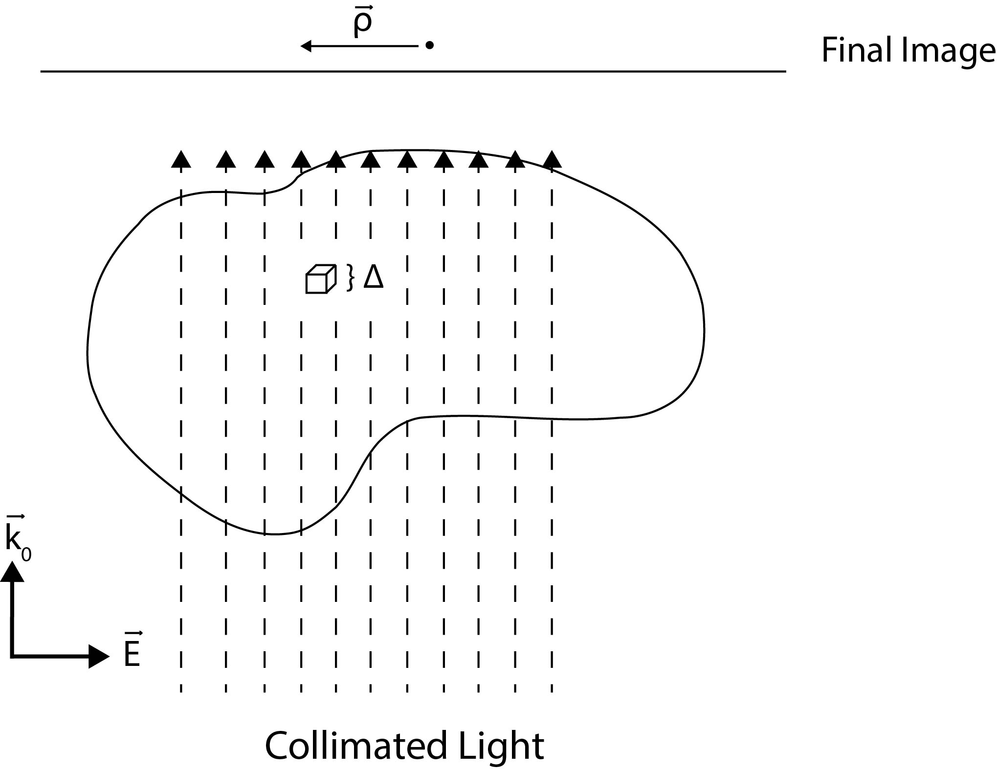
Fig. 3: An example showing how Jones Vectors and Matrices are used to propagate polarized states through birefringent elements. P_i and P_f are the initial and final polarization states and θ represents an optical element.

We take the goemetry we're interested in and fill it with the desired director field. Then we break the configuration up into volume elements of size Δ³. We want the size of each volume element to be small enough such that we can take the enclosed director to be constant. This allows us to treat each cube as a discrete optical element.

Now we can use Jones Calculus to determine the net effect of all the optical elements along an incident ray of light. After the light has passed through the analyzer, the final intensity is recorded on the output texture. We then repeat this process for all the rays passing through the bulk.

Thus, $$I(\vec{\rho}) = ||\hat{\Theta}_A \, \hat{\vartheta}(\vec{\rho}) \, \vec{E}_P||, $$ where $ \rho $ is the position vector in the output image, $ I(\vec{\rho}) $ is the intensity in the output image, $ \vec{E}_P$ is the initial polarization state of the light ray, $ \hat{\Theta}_A $ is the analyzer, and $ \hat{\vartheta}(\vec{\rho}) $ is the operator for a series of optical elements along the ray passing through $\rho$. In terms of the individual elements, $$ \hat{\vartheta}(\vec{\rho}) = \hat{\Theta}(\vec{\rho})_N\hat{\Theta}(\vec{\rho})_{N-1} \cdots \hat{\Theta}(\vec{\rho})_1 = \prod_{i = 1}^{N(\vec{\rho})}\!\hat{\Theta}(\vec{\rho})_i\, ,$$ where $ \hat{\Theta}(\vec{\rho})_i$ is the operator for the optical element associated with the i^th Δ ³ volume element along the ray.

Fig. 4: Fig 4: Simulation schematic. The bulk is broken into volume elements of Δ³ and a director value is assigned to each element. Light is then passed through the bulk in rays and the effect of each volume element on the polarization is computed. The final state is passed through the analyzer and the output intensity is recorded to create the final image. ρ refers to the position vector in the final texture.

[1] E. Pairam, et al., Stable nematic droplets with handles, PNAS. (2013) 110, 9295-9300
[2] Ondris-Crawford R, et al., Microscope textures of nematic droplets in polymer dispersed liquid crystals. J Appl. Phys. (1991) 69, 6380-6386

Soft Condensed Matter Laboratory, School of Physics, Georgia Institute of Technology
770 State Street NW, Atlanta, GA, 30332-0430, USA
Phone: 404-385-3667 Fax: 404-894-9958
alberto.fernandez [at] physics.gatech.edu