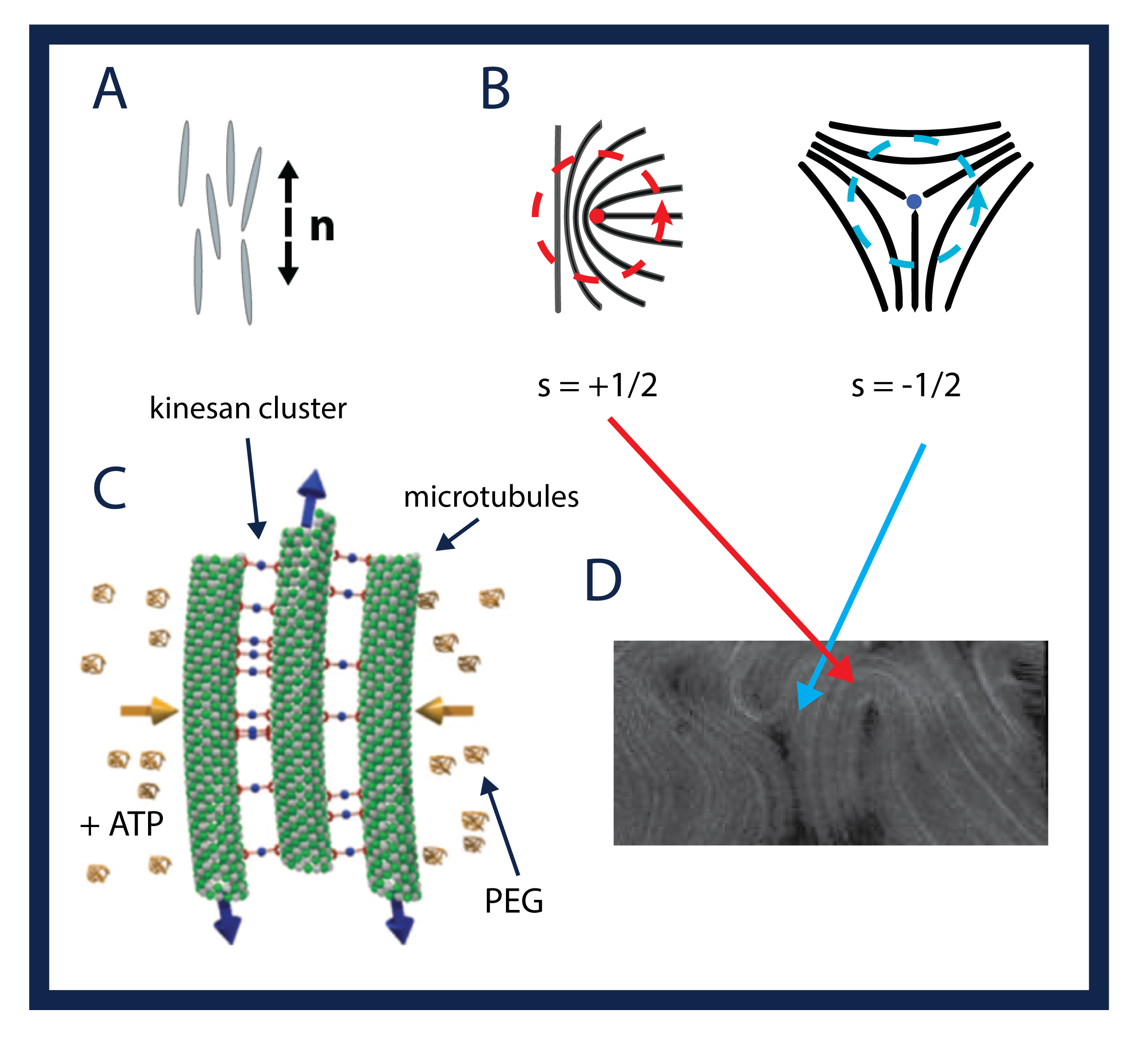
Nematics are generally composed of rod-like molecules that prefer to align with their long axes in the same direction. We use the director n to describe this local average orientation of a group of molecules, as seen schematically in Figure 1A. Places in the nematic where n is undefined are called defects, as shown schematically by the colored dots on the director diagrams in Figure 1B. Defects are characterized by their topological charge, \(s\) which is calculated using the director rotation along a closed path encircling the defect. For example, n rotates by &pi CCW along the red path in Figure 2B, giving \(s = +1/2\), and n rotates by -&pi CCW along the blue path in Figure 2B, giving \(s = -1/2\). The nematic system in this work is detailed schematically in Figure 1C. The individual rod-like units are microtubules. The activity comes from kinesan clusters that consume ATP and drive the microtubules to slide along each other. In this way the system has it's own source of internal energy and will never come to rest. The addition of PEG to the system causes the microtubules to deplete to each other and bundle together to form fibers. The depletion then drives these bundles to an interface to form a 2D nematic. The microtubules are fluorescently labeled, so we image to active nematic using fluorescent and confocal fluorescent microscopy. An example image with an \(s=+1/2\) and \(s=-1/2\) defect highlighted is shown in Figure 1D.

Fig. 1: (A), schematic demonstrating the director as a local average of the orientation of the NLC molecules. (B), director schematics of a +1/2 defect and a -1/2 defect. (C), the active nematic system. The fluorescently-labeled microtubules are the "molecules" of the active nematic. The activity comes from the kinesan clusters that consume ATP and cause the microtubules to slide by each other, as indicated by the blue arrows. The PEG acts a depletant, causing the microtubules to bundle together, as indicated by he yellow arrows. (D) A fluorescence image of an active nematic with a +1/2 and -1/2 defect indicated with the respective arrows.

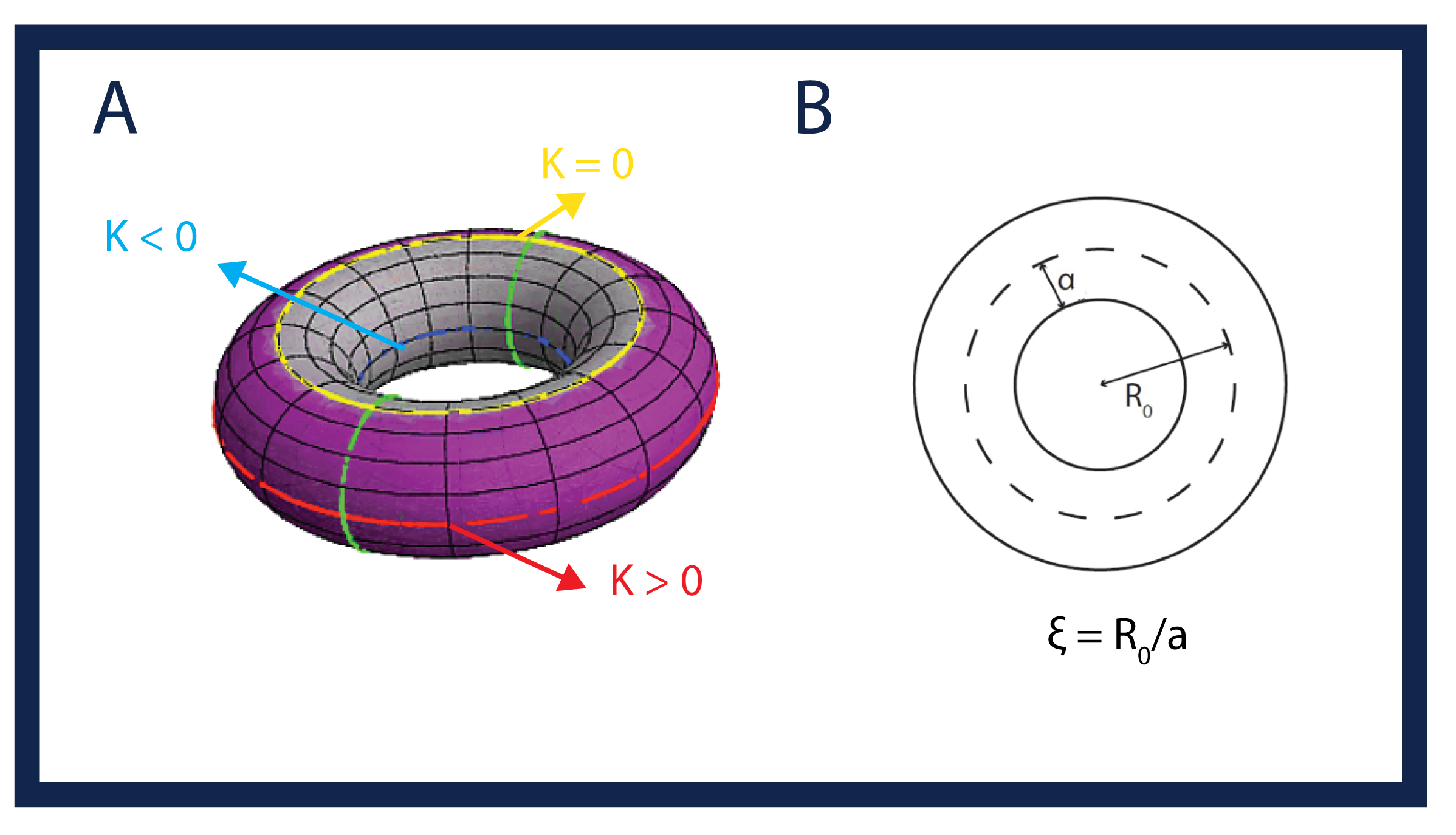
We put the active nematic on the surface of a toroid to explore the relationship between the Gaussian curvature, \(K\), and the defects. Theory predicts that the defects couple to \(K\) with \(s>0\) defects attracted to regions of \(K>0\) and \( s < 0 \) defects attracted to regions with \(K < 0 \). Toroids have positive \(K\) on the outside of the handle and negative \(K\) on the inside of the handle, as illustrated in Figure 2A. We characterize our toroids by their aspect ratio, \( \xi = R_0/a \), as defined schematically in Figure 2B.

The Experiment

Once the active nematic is depleted to the surface of a toroid, we image the sample using a confocal microscope. A z-scan of a confocal stack of a toroid at a single instant in time is found in Figure 3A. Note how most of the signal comes from just the surface. A rotation of the confocal stack showing that we are truly looking at the bottom half of the toroid in seen in Figure 3B.

Fig. 2: (A), schematic of a torus with the region of positive Gaussian curvature, \((K)\), in purple, the region of negative \(K\) in gray, and the \(K = 0\) line in yellow. The red line and the purple line represent the contours of maximum and minimum K, respectively. (B), top-down drawing of a torus defining the central circle radius, \(R_0\), the tube radius \(a\), and the aspect ratio \(\xi = R_0/a\).

A (video): Z-scan of a confocal stack	B (video): Rotating a confocal stack.
Fig 3: An active nematic on the surface of a toroid viewed through a confocal microscope.

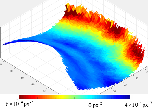
We image the toroid over time until the activity stops. An intensity projection of a sample dataset can be seen in Figure 4A. Note how the nematic never comes to rest and there is a constant creation and annihilation of defects. We use Coherence-Enhanced Diffusion Filtering to determine the director on the torus for every time step. Once we have the director, we find the defects; the director and defects for the example toroid seen in Figure 4A are plotted on top of the intensity projection and are found in Figure 4B. The defect tracks are displayed for each defect in the sample. We also measure the Gaussian curvature for each toroid by fitting the Weingarten Matrix everywhere on the surface; the Gaussian curvature for he example toroid in Figure 1A is seen in Figure 1C.

A (video): Intensity projection of an active nematic over time.	B (video): Director and defects plotted on an intensity projection of an active nematic over time.	C: Measured Gaussian curvature.
Fig 4: An active nematic on the surface of a torus viewed over time. From the raw intensity image in (A) we find the director and defects shown in (B). We also measure the Gaussian curvature of the surface, as seen in (C).

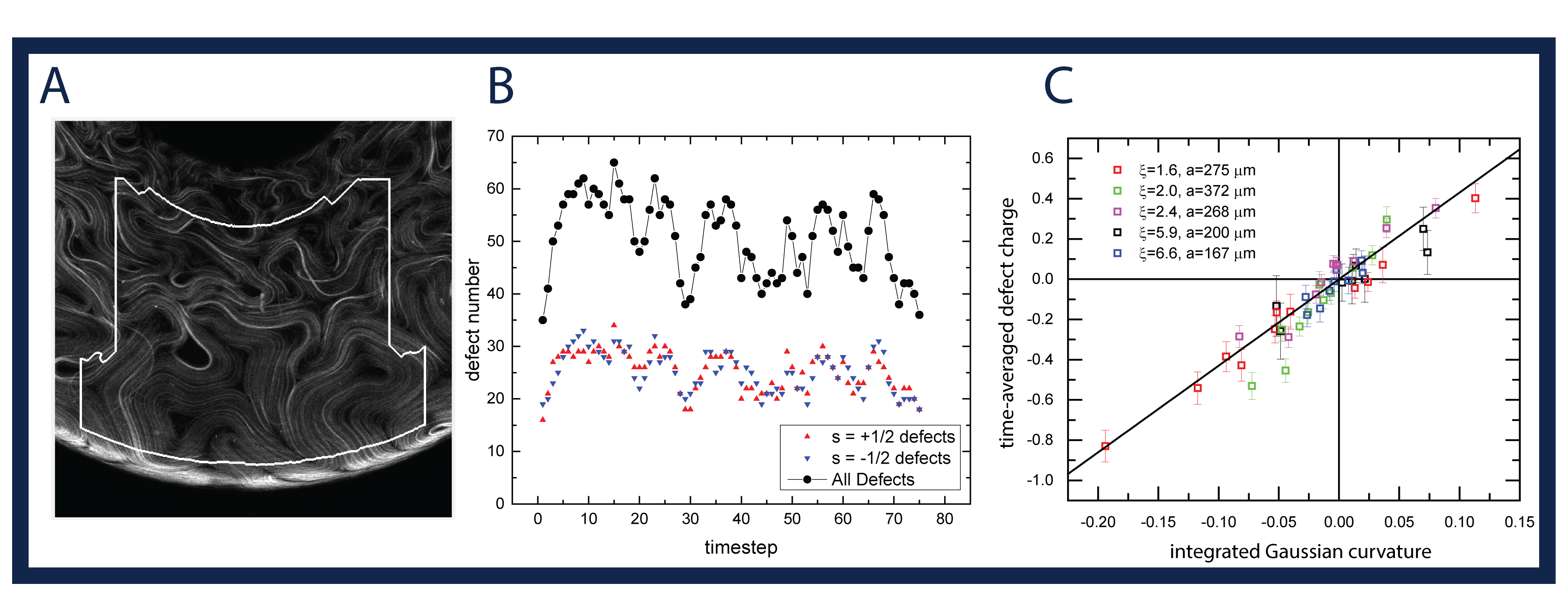
Results

We compare the topological charge in a region with its integrated Gaussian curvature. For the example image in Figure 5A, the region encircled in white has \(\int K = 0\). Since the defect number and topological charge in the region varies over time, as seen in the plot of total defect number and number of positive/negative defects over time in Figure 5B, we look at the time-averaged charge. In this example, \(\bar{s}=0\). When we compare these quantities for multiple regions over different toroids with different aspect ratio and size, the data collapse to a line, as seen in Figure 5C. This means that the time-averaged charge doesn't depend on the size of the region nor on how we draw the boundary of the region --- the only thing that matters is the integrated Gaussian curvature. In addition, there are on average more positive defects in regions of positive \(K\) and there are on average more negative defects in regions of negative \(K\) --- this means that we see the defects coupling to curvature and unbinding.

Fig. 5: (A), An image of an active nematic on the surface of a toroid. The area enclosed by the white border has \(\int K = 0 \). (B), the defect number over time for the region enclosed in white in (A). (C), Time-averaged defect charge vs integrated K in a set of regions for different toroids with different aspect ratios and tube radii. The line is an average of a linear fit to the data for each toroid and has a slope of \( 4.3 \pm 0.7 \).